Updated link for the National Fuel Moisture Database
The National Fuel Moisture Database is up and running. Please find it here: https://www.wfas.net/nfmd/public/index.php
Updating WFAS
A new WFAS is in the works. We are working behind the scenes to refresh WFAS and it's associated web presence. Keep checking for more updates.
02 Aug 2023
Welcome to WFAS
Forecast Fire Danger Conditions for today across the Continental United States
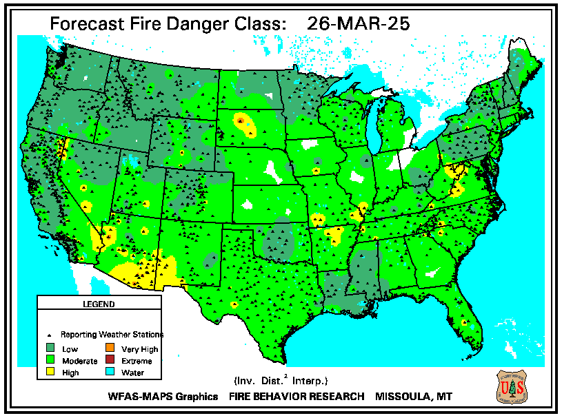
The Wildland Fire Assessment System (WFAS) is an integrated, web-based resource to support fire management decisions. It has an extensive nationwide user base of federal, state and local land managers. The system provides multi-temporal and multi-spatial views of fire weather and fire potential, including fuel moistures and fire danger classes from the US National Fire Danger Rating System (NFDRS), Keetch-Byram and Palmer drought indices, lower atmospheric stability and satellite-derived vegetation conditions. It also provides fire potential forecasts from 24 hours to 30 days. Point data for many products are provided in addition to spatial data for more localized applications. WFAS is under revision to refine existing products and to increase the utility of more spatial data products such as gridded surface meteorology and MODIS satellite data. Many of these new products will incorporate internet mapping services to allow users to resolve spatial products to a region of interest. These revisions will also provide higher resolution data for regional and local applications with higher spatial and temporal resolution. Planned changes will support decisions made at national, regional and local levels.